R package to understand overlap between multiple data frames and the implications of different types of joins.
Getting started
library(combineR)
library(tidyverse) # most useful with the tidyverse
#> ── Attaching packages ─────────────────────────── tidyverse 1.2.1 ──
#> ✔ ggplot2 3.0.0          ✔ purrr   0.2.5
#> ✔ tibble  1.4.2          ✔ dplyr   0.7.5.9000
#> ✔ tidyr   0.8.1          ✔ stringr 1.3.1
#> ✔ readr   1.1.1          ✔ forcats 0.3.0
#> ── Conflicts ────────────────────────────── tidyverse_conflicts() ──
#> ✖ dplyr::filter() masks stats::filter()
#> ✖ dplyr::lag()    masks stats::lag()
explain_rows
explain_rows gives the total number of rows, unique rows, and columns in each data frame:
explain_NAs
explain_NAs gives a report of nas in a data set
explain_NAs(math)
#> [[1]]
#> [1] "Here are the NA values in each column of the given dataframe, you have 24000 total rows in your dataset"
#>
#> [[2]]
#>   number_of_NA_values            variable percentage_of_total_dataset
#> 1                4761          math_score                       19.84
#> 2                   0          student_id                        0.00
#> 3                   0                year                        0.00
#> 4                   0 learning_disability                        0.00
#>
#> [[3]]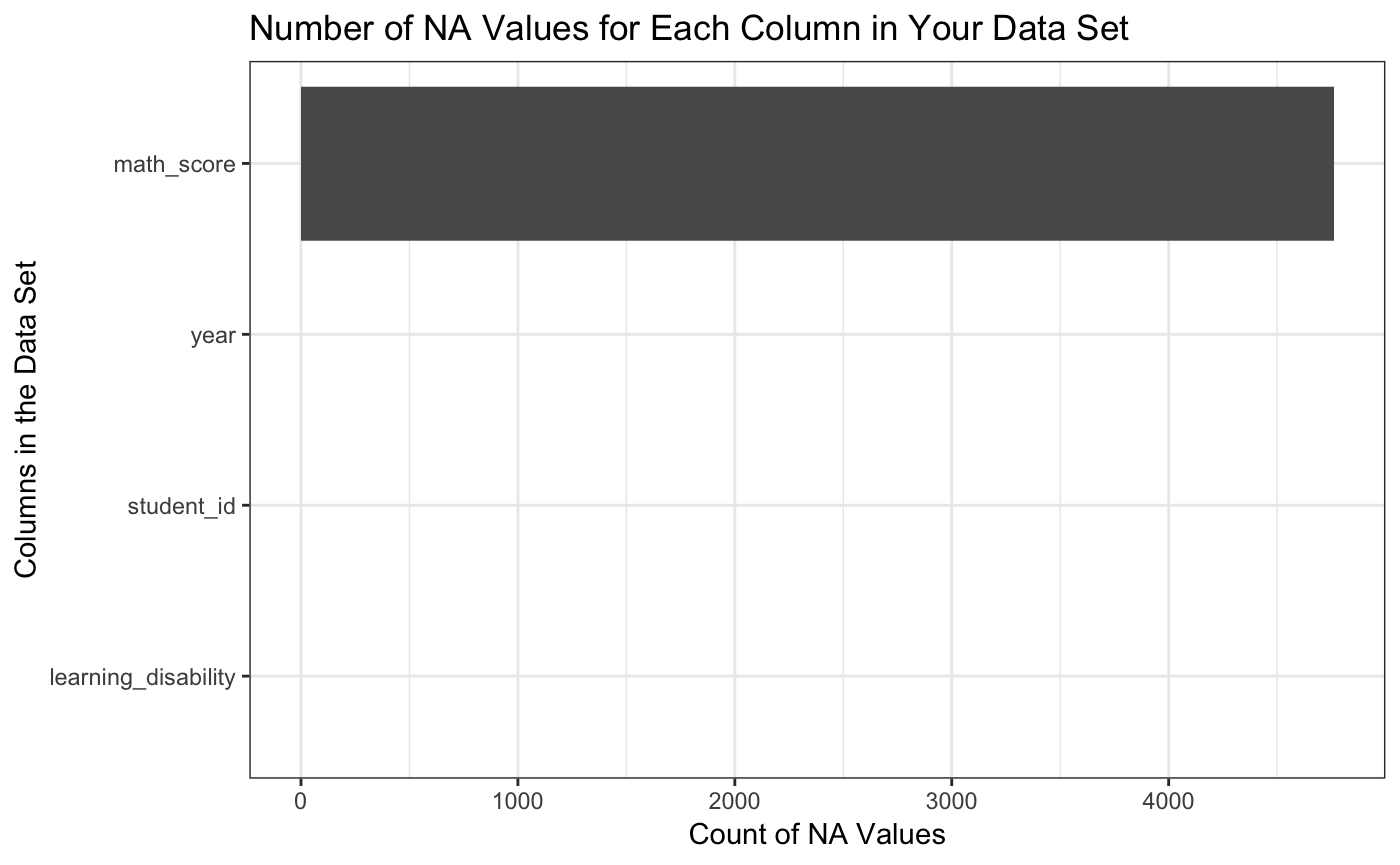
#>
#> [[4]]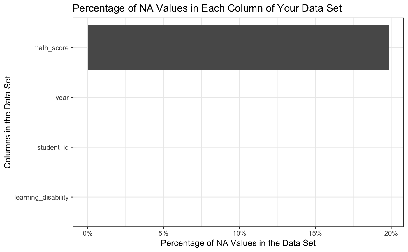
count_keys
The next function is count_keys. You give this as many data frames as you want and the key and it tells you how many unique values are in each data frame for the keys you specify. Here it is done for all three available datasets.
count_keys(demographics, math, ell, keys = c("student_id", "year"))
#> # A tibble: 30,000 x 5
#>    student_id  year demographics  math   ell
#>    <chr>      <dbl>        <int> <int> <int>
#>  1 S1000227    2015            1     1     0
#>  2 S1000227    2016            1     0     0
#>  3 S1000227    2017            1     1     0
#>  4 S1002738    2015            1     1     0
#>  5 S1002738    2016            1     1     0
#>  6 S1002738    2017            1     1     0
#>  7 S1003071    2015            1     1     0
#>  8 S1003071    2016            1     0     0
#>  9 S1003071    2017            1     1     0
#> 10 S100408     2015            1     0     0
#> # ... with 29,990 more rows
get_all_missing
When we do joins, there are two types of missing values that come up. The first are missing values that are hard coded. The second are missing values that are generated when we do a join.
The get_all_missing function lets you specify all of the data frames that you are interested in. You specify the keys (each data frame must have at least one of the keys in it). And then it tells you if you were to do all full_joins, in which variables you would see missing values and if they would come from being hard coded or from the join.
This function outputs a table and two plots to visualize the information. Here, we chose to visualize the combination of all three given datasets.
get_all_missing(demographics, math, ell, keys = c("student_id", "year"))
#> [[1]]
#> # A tibble: 9 x 3
#>   variable                         coded_missing join_missing
#>   <chr>                                    <int>        <int>
#> 1 name_demographics                            0            0
#> 2 sex_demographics                             0            0
#> 3 learning_disability_demographics             0            0
#> 4 learning_disability_math                     0         6000
#> 5 math_score_math                           4761         6000
#> 6 name_ell                                     0        20517
#> 7 sex_ell                                      0        20517
#> 8 learning_disability_ell                      0        20517
#> 9 ell_score_ell                             2904        20517
#>
#> [[2]]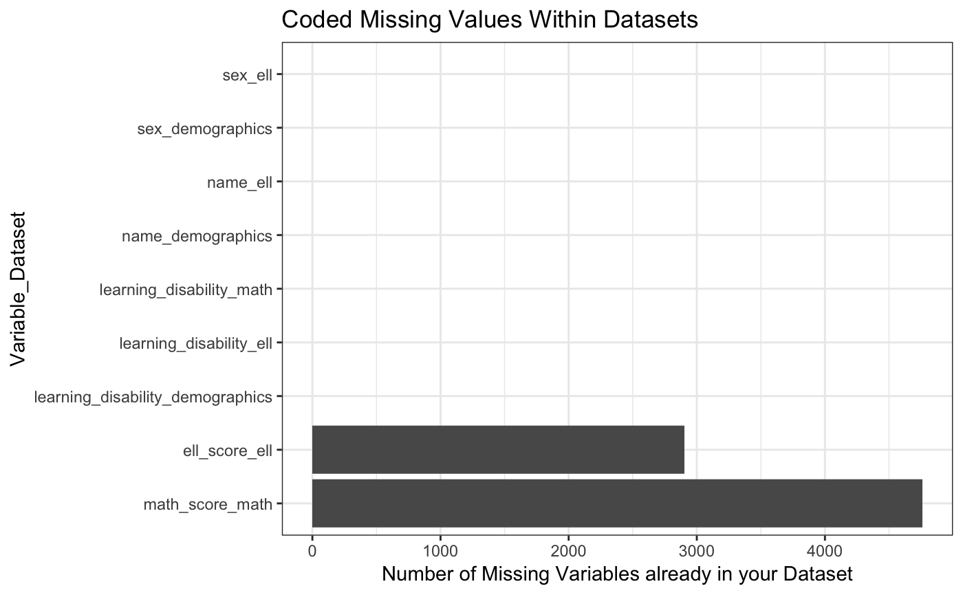
#>
#> [[3]]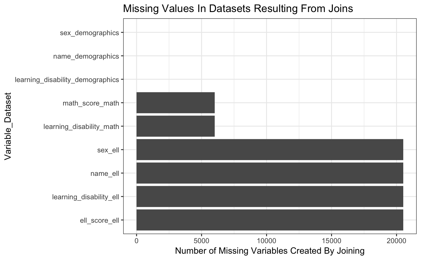
Example insights
The goal of combineR is to generate insights like the following:
There are a total of X unique students in the data.
Y% of students in demographic data are in the ell data while Z% of students in the state test data are in the math data.
If we want to create a completely non-missing dataset that includes gender and age from state demographics data, ell score and student id from ell data, and math score from the math data this will include XX students. YY students were dropped because they were in the demographic data but in neither of the other data sets. ZZ students were in all three data frames but had an NA in the math score variable from the math data.